Bayesian Methods for Hackers

3 minute read

1. 베이지안 추론의 철학

서론
- 사전확률 : 사건 A에 대한 우리의 믿음의 양
  $P(A)$
- 사후확률 : 증거 X가 주어진 상황에서 A의 확률
  $P(A|X)$
베이지안 프레임워크
- 베이즈 정리
  $P(A|X) = \frac {p(A)p(X|A)}{p(X)}$
확률분포
- 확률변수 Z가 이산적인 경우, 확률질량함수
  $P(Z=k) = \frac {\lambda^k e^{-\lambda}}{k!}$, $k=0,1,2,…$
  $Z$ ~ $Poi(\lambda)$
  $E[Z|\lambda] = \lambda$
- 확률변수 Z가 연속적인 경우, 확률밀도함수
  $f_Z(z|\lambda) = \lambda e^{-\lambda z}, z \ge 0$
  $Z$ ~ $Exp(\lambda)$
  $E[Z|\lambda] = \frac {1}{\lambda}$
컴퓨터를 사용하여 베이지안 추론하기
- PyMC를 사용한 베이지안
결론
부록
연습문제
참고자료

서론
- Stochastic 변수 : 값이 정해지지 않은 변수
- Deterministic 변수 : 변수의 부모를 모두 알고있는 경우에 랜덤하지 않은 변수
  - @pymc.deterministic 파이썬 래퍼 (데코레이터)를 써서 구분
모델링 방법
- 관측된 빈도와 실제 빈도간에는 차이가 발생
- 베르누이 분포
  $X$ ~ $Berp(p)$ : X는 p의 확률로 1, 1-p의 확률로 0
- 이항분포
  $X$ ~ $Bin(N, p)$
  $P(X=k)=\binom {n} {k} p^k (1-p)^{N-k}$
  기댓값 : $Np$
- 데이터 Import 예시
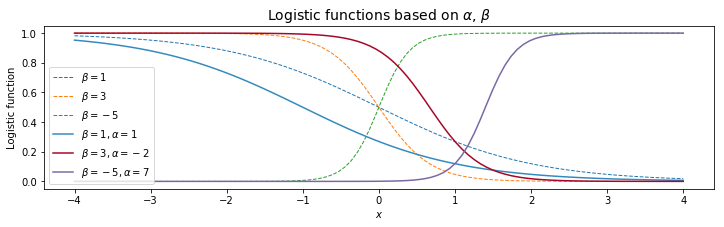
- Logistic Function
- 정규분포
  정규확률변수 : $X \sim N(\mu, 1/\tau)$
  확률밀도함수 : $f(x|\mu,\tau)=\sqrt{\frac {\tau}{2\pi}}exp(-\frac{\tau}{2}(x-\mu)^2)$
  정규분포의 기댓값 : $E[X|\mu, \tau]=\mu$
  정규분포의 분산 : $Var(X|\mu, \tau)=\frac{1}{\tau}$
우리의 모델이 적절한가?
결론
부록
연습문제
참고자료

서론
손실함수
$L(\theta, \hat{\theta}) = (\theta - \hat{\theta})^2$
$L(\theta, \hat{\theta}) = \cases {(\theta - \hat{\theta})^2 & ${\hat{\theta} \lt \theta}$ \cr c (\theta - \hat{\theta})^2 & ${\hat{\theta} \ge \theta, \;\; 0 \lt c \lt 1}$ }$
$L(\theta, \hat{\theta}) = |\theta - \hat{\theta}|$
$L(\theta, \hat{\theta}) = -\theta \log(\hat{\theta}) - (1 - \theta) \log(1 - \hat{\theta}), \;\; \theta \in {0, 1}, \; \hat{\theta} \in [0, 1]$
$l(\hat{\theta}) = E_{\theta} \left[ L(\theta, \hat{\theta}) \right]$
$\frac{1}{N} \sum_{i=1}^N L(\theta_i, \hat{\theta}) \approx E_{\theta} \left[ L(\theta, \hat{\theta}) \right] = l(\hat{\theta})$
베이지안 방법을 통한 기계학습
$R_i(x) = \alpha_i + \beta_ix + \epsilon$
where $\epsilon \sim \text{Normal}(0, \sigma_i)$ and $i$ indexes our posterior samples.
$\arg \min_{r} E_{R(x)} \left[ L(R(x), r) \right]$
- 예제: 금융예측
결론
참고자료

서론
주관적인 사전확률분포 vs. 객관적인 사전확률분포
$\mu_p = \frac{1}{N} \sum_{i=0}^N X_i$
알아두면 유용한 사전확률분포
- 감마분포
  $\text{Exp}(\beta) \sim \text{Gamma}(1, \beta)$
  $F(x \mid \alpha, \beta) = \frac{\beta^{\alpha}x^{\alpha - 1}e^{-\beta x}}{\Gamma(\alpha)}$
- 베타분포
  $f_X(x | \alpha, \beta) = \frac{x^{(\alpha - 1)}(1 - x)^{(\beta - 1)}}{B(\alpha, \beta)}$
  Observation : $X \sim \text{Binomial}(N, p)$
  Posterior : $\text{Beta}(1 + X, 1 + N - X)$
예제: 베이지안 MAB (Multi-Armed-Bandits)
해당 분야 전문가로부터 사전확률분포 유도하기
$w_{opt} = \max_{w} \frac{1}{N} \left( \sum_{i=0}^N \mu_i^T w - \frac{\lambda}{2}w^T\Sigma_i w \right)$
켤레 사전확률분포
제프리 사전확률분포
N이 증가할 때 사전확률분포의 효과
$p(\theta | {\textbf X}) \propto \underbrace{p({\textbf X} |\theta)}_{\textrm{likelihood}} \cdot \overbrace{p(\theta)}^{\textrm{prior}}$
$\log(p(\theta | {\textbf X})) = c + L(\theta; {\textbf X}) +\log(p(\theta))$
- 서로 다른 사전확률분포에서 시작하더라도 표본 크기가 증가함에 따라 사후확률분포는 수렴함
결론
부록
참고자료